Inventory Model Simulation

The overall objective of inventory (stock) control is to maintain inventory levels to that the total costs of holding stocks is minimise. A popular method of implementing stock control is through the use of inventory (stock) control charts and algorithms that automate the process.

Economic Order Quantity – EOQ Definition 

 

By Will Kenton
Reviewed By Janet Berry-Johnson
Updated Feb 10, 2020


What Is Economic Order Quantity (EOQ)?

Economic order quantity (EOQ) is the ideal order quantity a company should purchase to minimize inventory costs such as holding costs, shortage costs, and order costs. This production-scheduling model was developed in 1913 by Ford W. Harris and has been refined over time.1 The formula assumes that demand, ordering, and holding costs all remain constant.

The EOQ is a company's optimal order quantity that minimizes its total costs related to ordering, receiving, and holding inventory.
The EOQ formula is best applied in situations where demand, ordering, and holding costs remain constant over time.
Formula and Calculation of Economic Order Quantity (EOQ)

The formula for EOQ is:

​where: 

Q=EOQ units
D=Demand in units (typically on an annual basis)
S=Order cost (per purchase order)
H=Holding costs (per unit, per year)​

Matlab Simulation

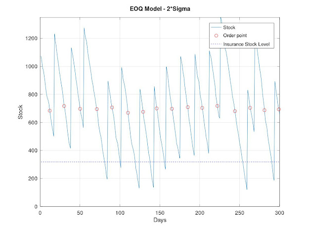
The Simulation descibe a 300 days of stock. Each time the stock is at an Order Point, an Order of constant quantity is ordered to wholesaler.

The Quntity of Consuming the stock and the supply days change randomally in normal distribution.

The model take safety stock equal 2*sigma where sigma is the standard deviation of multipliction of the random variables : stock consume per day and days of supply.

Inventory Model

Matlab Script:

% This Script Plot The Inventory Model of an item
pkg load statistics
clear

item_name = "Filter"

Main_ConsumePerDay = 40 % Main of items consume per day
Stdev_ConsumePerDay = 10 % Standard deviation of consume items per day

Main_SupplyDay = 10 % Main of the days to supply the item
Stdev_SupplyDay = 3   % Standard deviation of the days to supply the item

NumberDays = 300 % Number of days for simulation
N_STD = 2 % Number of standard deviation use for insurance inventory

% Calculate Quantity per Order
DaysPerYear = 250
interest_rate = 0.15 % The interest rate to hold stock

k = 300;    % Order Coast
item_price = 70 % Price of unit item
h = interest_rate * item_price  % price of holding one item per year
ConsumePerYear = DaysPerYear * Main_ConsumePerDay % Consume per Year

Optimal_QuntityOrder = round(sqrt(2*ConsumePerYear*k/h)); % Optimal Quntity Per Order
EOQ = Optimal_QuntityOrder % Economic Order Quantity
OrderExist = false

% Main consume during the supply period (in days)
MainConsumeSupplyDays = Main_ConsumePerDay*Main_SupplyDay

% standard ddeviation of consume during supply period
StdevConsumeSupplyDays = sqrt(Stdev_ConsumePerDay^2*Stdev_SupplyDay^2+
Stdev_ConsumePerDay^2*Main_SupplyDay^2+ Stdev_SupplyDay^2*Main_ConsumePerDay^2)

% Insurance inventory
InsureInventory = N_STD * StdevConsumeSupplyDays

% Order Point
OrderPoint = InsureInventory + MainConsumeSupplyDays %+ EOQ

StartStock = InsureInventory + EOQ

% Array of random consume per day of the utem
ConsumePerDayVal = normrnd(Main_ConsumePerDay, Stdev_ConsumePerDay,1, NumberDays);

stock(1) = StartStock;
i_order = 1 % index for order points
for i=1:NumberDays
  % Stock is under order point but no order yet
  if (stock(i) < OrderPoint) && (OrderExist == false)
    stock(i)
    OrderExist = true;
    j=1;
    N_SupplyDays = max(1, round(normrnd(Main_SupplyDay, Stdev_SupplyDay)))
    Xorder(i_order) = i;
    Yorder(i_order) = stock(i);
    i_order = i_order+1;
    
  % Stock is under order point and order exist
  elseif (stock(i) < OrderPoint)
    j=j+1;
    if (j-N_SupplyDays)>0.1
      OrderExist = false;
      stock(i) = stock(i) + EOQ;
    end
  end
  stock(i+1) = stock(i) - ConsumePerDayVal(i);

end

plot(stock(1:NumberDays))
axis([0 NumberDays 0 inf])
title('EOQ Model - 2*Sigma')
xlabel('Days')
ylabel('Stock')
hold
plot(Xorder, Yorder, 'ro')

grid
x(1:NumberDays) = 1:NumberDays;
y(1:NumberDays) = InsureInventory;

plot( y, 'b--')

legend('Stock','Order point', 'Insurance Stock Level')

 

Octave - Symbolic calculation - Plot function and its derivetive

This symbilic script get input a function f(x), and the order n of the derivetive requsted.
The script plot the function f(x) and the order n derivetive.

Download the file plot_derive_sym_order_n.m

% This script plot derivetive fd(x) of the function f(x).
% The script use the function_handle function to create numeric
% function ffd from dff(x).

pkg load symbolic
setenv PYTHON C:\ProgramData\Anaconda3\pythonw.exe

disp('Order of derivetive:')
n = 2
% Declare symbolic variable x
syms x;

disp('The function f(x):')
% Input the function f(x) here:
f = sin(x) + cos(x)+ x^2*sin(x)

disp('The n order derivetive fd(x) of the function f(x):')
% The derivative of the function f:
% fd(x) = f'(x)
fd(1) = diff(f,x);
i1 = 2;
while i1<=n
      fd(i1) = diff(fd(i1-1), x);
      i1++;
endwhile
fd(n)
% Convert symbolic function fd(x) to numeric function dff(x):
dff = function_handle(fd(n));

x=-2*pi:0.1:2*pi;
y= dff(x);
plot(x,y)
grid
xlabel('x')
ylabel('fd order n(x)')

Output

Symbolic derive of function and plot it

download file plot_derive_sym.m
Octave platform

% This script plot derivetive fd(x) of the function f(x).
% The script use the function_handle function to create numeric
% function ffd from dff(x).

pkg load symbolic
setenv PYTHON C:\ProgramData\Anaconda3\pythonw.exe

 % Declare symbolic variable x
syms x;

disp('The function f(x):')
% Input the function f(x) here:
f = sin(x) + cos(x)+ x*sin(x)

disp('The derivetive fd(x) of the function f(x):')
% The derivative of the function f:
% fd(x) = f'(x)
fd = diff(f, x)

% Convert symbolic function fd(x) to numeric function dff(x):
dff = function_handle(fd);

x=-2*pi:0.1:2*pi;
y= dff(x);
plot(x,y)
xlabel('x')
ylabel('fd(x)')

Output

>> plot_derive_sym
The function f(x):
f = (sym) x*sin(x) + sin(x) + cos(x)
The derivetive fd(x) of the function f(x):
fd = (sym) x*cos(x) + cos(x)

הוסף כיתוב

Octave - Use solve function to symbolic solution of equation whith one variable

Download file one_var_solve.m

% Script for solving equation with one variable using the solve function
% sytax :
% S = solve(eqn,var) solves the equation eqn for the variable var.

% load symbolic package, and initilize PYTHON variable. (Octave only).
pkg load symbolic
setenv PYTHON C:\ProgramData\Anaconda3\pythonw.exe

% Declare symbolic and variables and parameters
syms a b c x

% Define the equation to solve:
eqn = a*x^2 + b*x + c == 0

% activate solve function for x
S = solve(eqn, x)

% Solve for b:
Sb = solve(eqn, b)


Output

Octave - Create two Symbolic matrices and calculte thier product

The script declare symbolic variables: psi phi theta psidot phidot thetadot, and create 3 matrices RzPsi, RyTheta, RzPhiwith with the variables and print the matrices.

The script also calculate symbolic products of the matrices RzPhi * RyTheta,

and print the product. 

Download the file sym_mat.m

% script demonstrate how to use Symbolic matice

% load symbolic package, and initilize PYTHON variable. (Octave only).
pkg load symbolic
setenv PYTHON C:\ProgramData\Anaconda3\pythonw.exe

% Declare Symbolic variable
syms psi phi theta psidot phidot thetadot

% Define Symbolic matrices
RzPsi = [[cos(psi), -sin(psi), 0]; [sin(psi), cos(psi), 0]; [0,0,1]]
RyTheta = [[cos(theta), 0, sin(theta)];[0,1,0];[-sin(theta), 0, cos(theta)]]
RzPhi = [[cos(phi), -sin(phi), 0]; [sin(phi), cos(phi), 0]; [0,0,1]]

disp(' Calculate the symbolic products of: RzPhi * RyTheta')

% Multiply Symbolic Matrices
RzPhi * RyTheta

The script output:

Demo of inputting a function at the input prompt

The script get function at the prompt and calculate the first and the second order derivative
of the function. The script can be run on Octave platform.
Download the file demo_prompt_function.m

%     Demo of inputting a function at the input prompt
%     and making an Anonymous function.

% This program. shows how to take a
% string input and make it into an anonymous function
% this uses the symbolic pkg.
% Load Symbolic pkg (Octave only)
pkg load symbolic
setenv PYTHON C:\ProgramData\Anaconda3\pythonw.exe

disp("Example input")
disp("x^2 + 3*x - 1 + 5*x*sin(x)")
str_fucn=input("please enter your function  ","s")
fucn_sym=sym(str_fucn)
f=function_handle(fucn_sym)
% now back to symbolic
syms x;
ff=formula(f(x));
% now calculate the derivative of the function
ffd=diff(ff);
% and convert it back to an Anonymous function
df=function_handle(ffd)
% now lets do the second derivative
ffdd=diff(ffd);
ddf=function_handle(ffdd)
% and now plot them all at interva (-2) - 2
x1=-2:.001:2;
plot(x1,f(x1),x1,df(x1),x1,ddf(x1))
grid minor on
legend("f","f '", "f '' ")

The result for input function cos(x)

Example input
x^2 + 3*x - 1 + 5*x*sin(x)
please enter your function  cos(x)
str_fucn = cos(x)
fucn_sym = (sym) cos(x)
f =

@(x) cos (x)

df =

@(x) -sin (x)

ddf =

@(x) -cos (x)

The Graph

Octave - Calculate argument in Symbolic function

The script convert symbolic expression df(x) to funtion dfh(x) using the

 function_handle Octave function. The script can run on Octave platform.
Download the file demo_sym.m

% Demo of how to use a number (which was calculated in an octave
% variable) in a symbolic calculation, without getting a warning.

% use octave to calculate some number:
 a = pi/2

% now do some work with the symbolic pkg
 syms x
 f = x * cos (x)
 df = diff (f)

% Now we want to evaluate df at a:

 % subs (df, x, a)     # this gives the "rats" warning (and gives a symbolic answer)

% So instead, try

 dfh = function_handle (df)

 disp('dfh(a) = ')
 dfh (a)

% ans = -1.5708


% And you can evaluate dfh at an array of "double" values:

disp ('dfh ([1.23 12.3 pi/2]) = ')
 dfh ([1.23 12.3 pi/2])

% ans =
%  -0.82502   4.20248  -1.57080

The Result

a =  1.5708
f = (sym) x*cos(x)
df = (sym) -x*sin(x) + cos(x)
dfh =

@(x)   -x .* sin (x) + cos (x)

dfh(a) =
ans = -1.5708
dfh ([1.23 12.3 pi/2]) =
ans =

  -0.82502   4.20248  -1.57080

Matlab - Symbolic mulitiplication matrice by operator

The Script multiply operator matrice U by matrice A . The script run on octave platform.
Download the file matrice1.m

% This script define symbolic  4*4 matrix A
% The script define matrix U as opertor
% The script solve the multilication U*A

% Load symbolic package, and initilize PYTHON variable.
pkg load symbolic
setenv PYTHON C:\ProgramData\Anaconda3\pythonw.exe

% Define Symbolic variables
syms x11 x12 x13 x14 x21 x22 x23 x24
syms x31 x32 x33 x34 x41 x42 x43 x44

% Matrice A
A = [ x11 x12 x13 x14
x21 x22 x23 x24
x31 x32 x33 x34
x41 x42 x43 x44 ]

% Operator Matrice U
U = [ 0 0 0 0
1 0 0 0
1 1 0 0
0 0 0 0 ]

disp('C = U*A')
 C = U*A

The result

Matlab - Plot simple graph

Plot y = sin(x) graph (Octave platform)
Download the file simple_graph.m

% Simple y=sin(x) graph plot

x= 0:0.01:2*pi; % x Vector of x values
y = sin(x);     % y vector ' y = sin(x)

plot(x,y)       % Plot the graph y = sin(x)

% Add tiltles and grid
xlabel('x')
ylabel('sin(x)')
title('Graph - y = sin(x)')
grid

The Graph

Matlab Script - Symbolic solution for second-order differential equation

This Script run on Octave platform. The script get input second order differential equation with initial condition, of the form:

 The script return the function y(t).
Download the file simplediff2.m 

% Script to solve  second-order differential equation

% Specify the second-order derivative by using:
% diff and the equation by using ==.
% Then, solve the equation by using dsolve.

% load symbolic package, and initilize PYTHON variable
pkg load symbolic
setenv PYTHON C:\ProgramData\Anaconda3\pythonw.exe

% Define symbolic variables:
% y(t) - function y and argumenr t
% a - parameter
% y0 - initial condition for y(t) -  y(0) = y0
% y1 - initial condition for y'(t) -  y'(0) = y1

syms y(t) a y0 y1

% ****  input the equaion here: *****
eqn = diff(y,t,2) == a*y;

% S = dsolve(eqn, cond)
S = dsolve (eqn, y(0) == y0, diff(y)(0) == y1)

Example :

Differential equation with initial condition:

% ****  input the equaion here: *****
eqn = diff(y,t,2) == a*y;

% S = dsolve(eqn, cond)
S = dsolve (eqn, y(0) == y0, diff(y)(0) == y1)

The Solution:

Matlab Script - Symbolic solution for first-order differential equation

This Script run on Octave platform. The script get input differential equation with initial condition, of the form:
 

 The script return the function y(t).
 Download the file simplediff1.m 

% simple script to solve
% Symbolic solution for first-order differential equation

% Specify the first-order derivative by using:
% diff and the equation by using ==.
% Then, solve the equation by using dsolve.

% load symbolic package, and initilize PYTHON variable
pkg load symbolic
setenv PYTHON C:\ProgramData\Anaconda3\pythonw.exe

% Define symbolic variables:
% y(t) - function y and argumenr t
% a - parameter
% y0 - initial condition for y(t) -  y(0) = y0

syms y(t) a y0 t0
% ****  input the equaion here: *****
eqn = diff(y,t) == a*y;

% ****  input the initial conditions here: *****
cond = [y(0)==y0];

S = dsolve(eqn, cond)

Examples 1:

Differential equation with initial condition:

 % ****  input the equaion here: *****
eqn = diff(y,t) == a*y;
% ****  input the initial conditions here: *****
cond = [y(0)==y0];

 The solution:

                                                                                                  

Examples 2:

Differential equation with initial condition:

% ****  input the equaion here: *****
eqn = diff(y,t) == a*t*y;

% ****  input the initial conditions here: *****
cond = [y(0)==y0];

 The solution:

Examples 3:

% ****  input the equaion here: *****
eqn = diff(y,t) == a*y;
% ****  input the initial conditions here: *****
cond = [y(t0)==y0];

 The solution: